
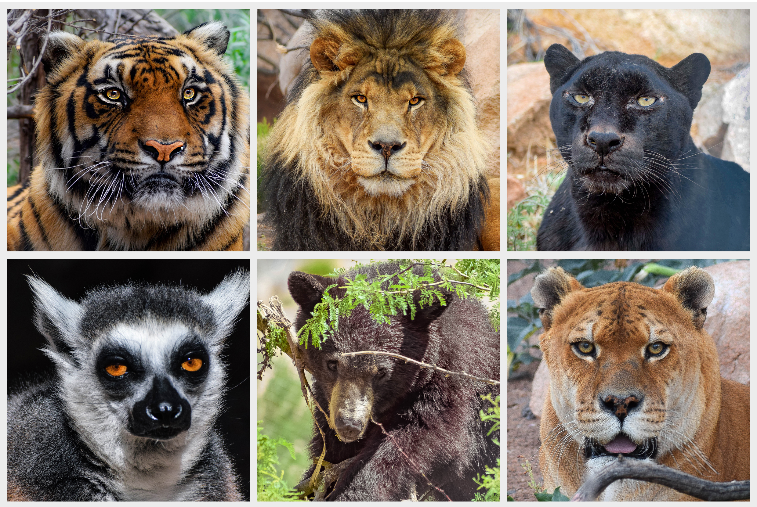
 Pic Credit: https://www.globalgiving.org/projects/help-feed-rescued-wild-animals-in-arizona/
Image classification is one of the supervised machine learning problems which aims to categorize the images of a dataset into their respective categories or labels. We can use traditional machine learning classification algorithms on hand-crafted image features or train end-to-end deep learning models to classify the images. This blog covers the basic explanation of traditional machine learning algorithms like K-Nearest Neighbor(KNN) , Naive Bayes, Random Forest and Support Vector Machine(SVM) along with introduction to deriving image features using Bag of Visual Words, followed by using pre-trained deep learning models and using transfer learning. Specifically, we will look at the implementation of multi class image classifier using Transfer learning on pre-trained Inception-ResNet-V2 and also using image features (Bag of Visual Words) with traditional algorithms like KNN, Naive Bayes, Random Forest and Support Vector Machine classifiers for Wild Animals Images Dataset (Kaggle) [1]. Also, we will look into the performance comparison of the implemented models.
This sections provides a brief explanation of the traditional machine learning algorithms like KNN, Naive Bayes, Random Forest and SVM, and Deep Learning technique called Transfer Learning. Also, provides the advantages and disadvantages of each algorithm.
K Nearest Neighbor is one of the supervised machine learning algorithms used for classification. It classifies the data point based on its K neighbors classification.K-nearest neighbors (KNN) algorithm calculates the similarity of new data point with the data points in training set and assigns label to the new data point based on the labels of its first K neighbors.
Initially, load the training as well as test data.Then, we need to choose the value of K i.e. the nearest data points. K can be any integer.Next,For each point in the test data calculate the distance between test data and each row of training data with the help of any of the method namely: Euclidean, Manhattan or Hamming distance. The most commonly used method to calculate distance is Euclidean. Now, based on the distance value, sort them in ascending order.Next, it will choose the top K rows from the sorted array.and will assign a class to the test point based on most frequent class of these rows.[2]
pic credit:https://www.datacamp.com/tutorial/k-nearest-neighbor-classification-scikit-learn

Naive Bayes classifier is a machine learning classification algorithm based on Bayes Theorem. Naive Bayes classification algorithm assumes that the given features are independent of each other. When working with continuous data, an assumption often taken is that the continuous values associated with each class are distributed according to a normal (or Gaussian) distribution. This leads to Gaussian Naive Bayes classifier[4]. The likelihood of the features is assumed to be-
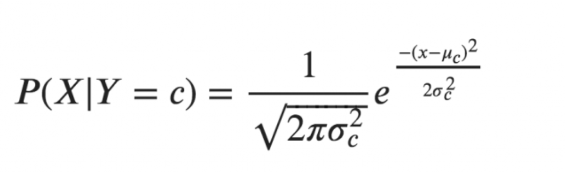 In the above formula, sigma is the variance and mu is the mean of the continuous variable X computed for a given class c of Y. The above formula calculated the probabilities for input values for each class through a frequency. We can calculate the mean and standard deviation of x’s for each class for the entire distribution.This means that along with the probabilities for each class, we must also store the mean and the standard deviation for every input variable for the class.
mean(x) = 1/n * sum(x)
where n represents the number of instances and x is the value of the input variable in the data.
standard deviation(x) = sqrt(1/n * sum(xi-mean(x)^2 ))
Here square root of the average of differences of each x and the mean of x is calculated where n is the number of instances, sum() is the sum function, sqrt() is the square root function, and xi is a specific x value.
Random forest is a Supervised Machine Learning Algorithm that is used widely in Classification and Regression problems. It builds decision trees on different samples and takes their majority vote for classification and average in case of regression.One of the most important features of the Random Forest Algorithm is that it can handle the data set containing continuous variables as in the case of regression and categorical variables as in the case of classification. It performs better results for classification problems [6] . 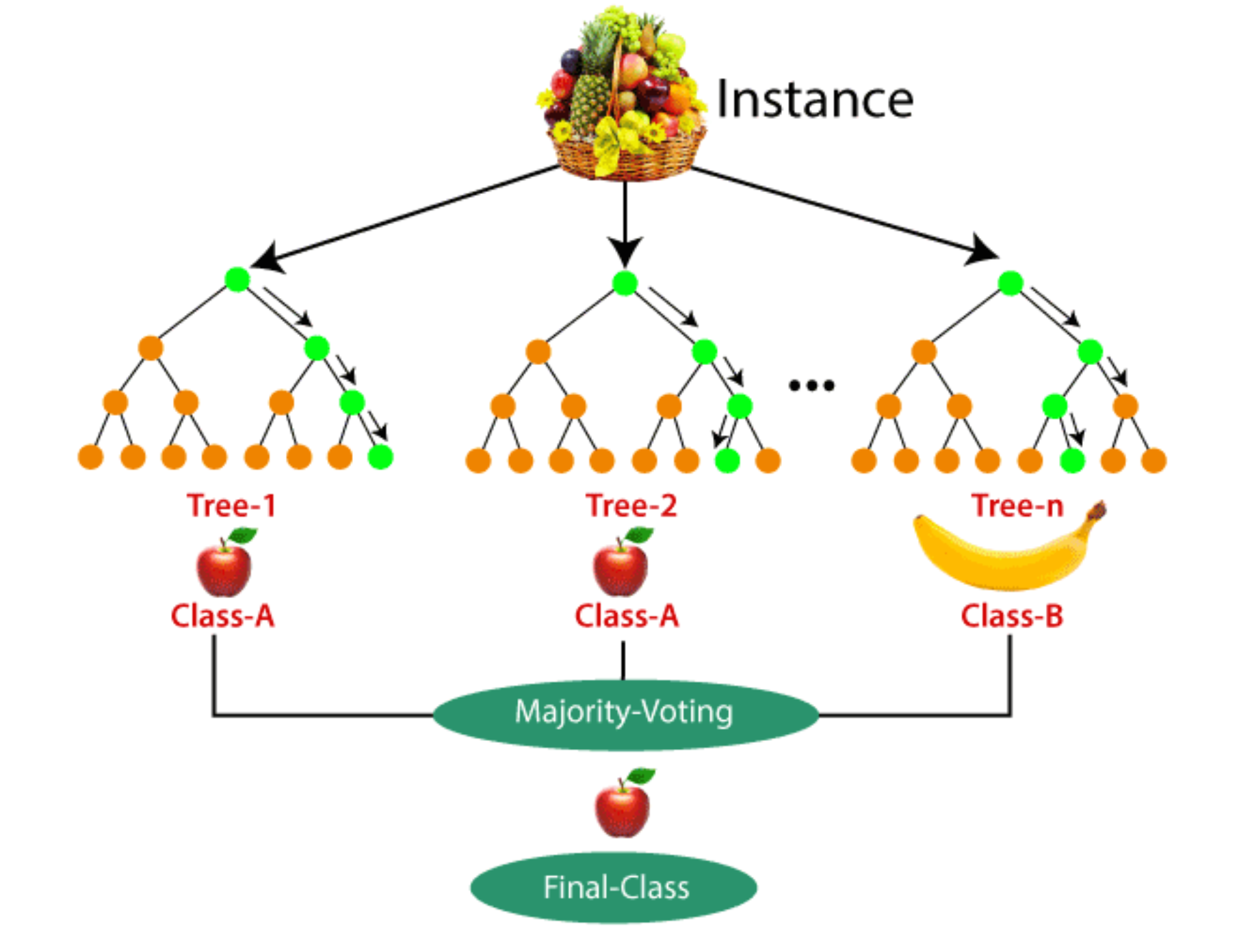
The critical difference between the random forest algorithm and decision tree is that decision trees are graphs that illustrate all possible outcomes of a decision using a branching approach. In contrast, the random forest algorithm output are a set of decision trees that work according to the output.In the real world, machine learning engineers and data scientists often use the random forest algorithm because they are so accurate and because modern computers and systems can usually handle large, previously unmanageable datasets.[7]
The objective of the support vector machine algorithm is to find a hyperplane in an N-dimensional space(N — the number of features) that distinctly classifies the data points. To separate the two classes of data points, there are many possible hyperplanes that could be chosen. Our objective is to find a plane that has the maximum margin, i.e the maximum distance between support vectors of both classes. Maximizing the margin distance provides some reinforcement so that future data points can be classified with more confidence.
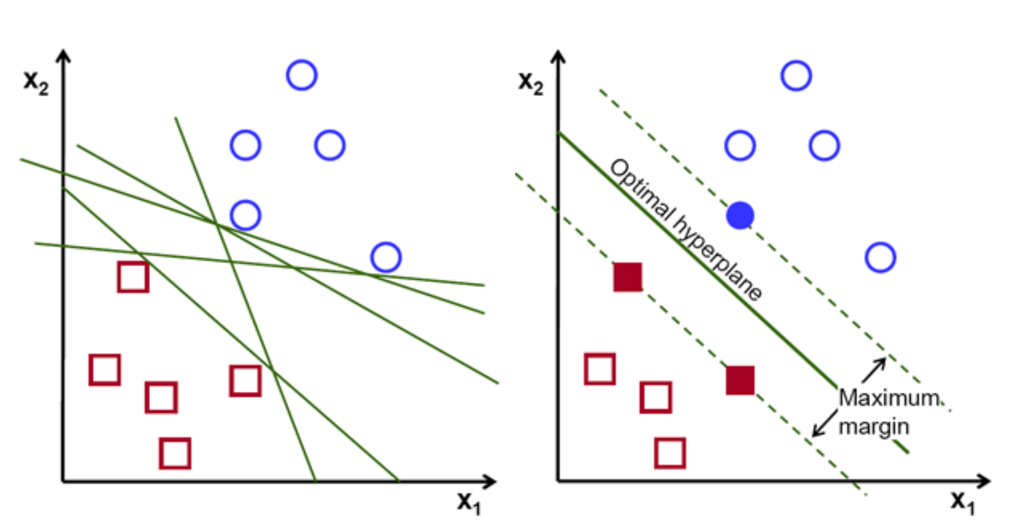 Support vectors are data points that are closer to the hyperplane and influence the position and orientation of the hyperplane. Using these support vectors, we maximize the margin of the classifier. Deleting the support vectors will change the position of the hyperplane. These are the points that help us build our SVM.
Transfer learning is a popular deep learning method that follows the approach of using the knowledge that was learned in some task and applying it to solve the problem of the related target task. So, instead of creating a neural network from scratch we “transfer” the learned features which are basically the “weights” of the network. To implement the concept of transfer learning, we make use of “pre-trained models“.
Pre-trained models are the deep learning models which are trained on very large datasets, developed, and are made available by other developers who want to contribute to this machine learning community to solve similar types of problems. It contains the biases and weights of the neural network representing the features of the dataset it was trained on. The features learned are always transferable. For example, a model trained on a large dataset of flower images will contain learned features such as corners, edges, shape, color, etc.
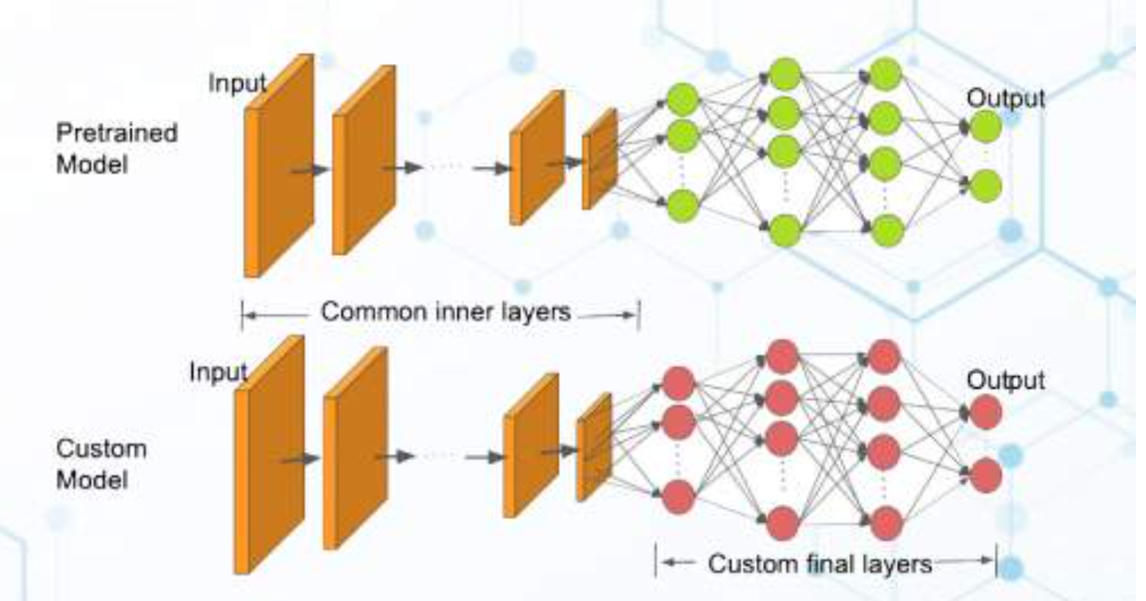
The intuition behind transfer learning for image classification is that if a model is trained on a large and general enough dataset, this model will effectively serve as a generic model of the visual world. You can then take advantage of these learned feature maps without having to start from scratch by training a large model on a large dataset.
InceptionResNetV2 is a convolutional neural network that is 164 layers deep, trained on millions of images from the ImageNet database, and can classify images into more than 1000 categories such as flowers, animals, etc. The input size of the images is 299-by-299.
This blog uses Wild Animals Image Dataset from kaggle (Wild Animals Image Dataset).
This dataset contains six different wild animals images with three different sizes(224 x 224 , 300 x 300, 512 x 512) in eighteen directories. Each directory contains wild animal images with animal name and size itself. This blog uses wild animals images with 300 x 300 size.
The following directories are used in this blog
1. cheetah-resize-300 - Contains cheetah images with size 300 x 300
2. fox-resize-300 - Contains fox images with size 300 x 300
3. hyena-resize-300 - Contains hyena images with size 300 x 300
4. lion-resize-300 - Contains lion images with size 300 x 300
5. tiger-resize-300 - Contains tiger images with size 300 x 300
6. wolf-resize-300 - Contains wolf images with size 300 x 300
The above data directories are segregated into following two directories and Remove the invalid image files from the directories.
1.train_size_300 - This directory contains 6 sub directories with animal name itself. Each directory contains 70% of the respective data.
2.valtest_size_300 - This directory contains 6 sub directories with animal name itself. Each directory contains 30% of the respective data.
The main goal of this blog is to build multi class image classifier using Transfer Learning on pre-trained Inception-ResNet-V2 and also using image features (Bag of Visual Words) with traditional algorithms like KNN, Naive Bayes, Random Forest and Support Vector Machine classifiers for Wild Animals Images Dataset (Kaggle) [1].
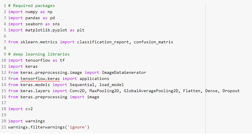
Import the required packages
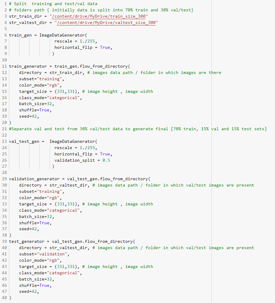
1. Load datasets and split the dataset into training and test/val data
2. Load base model (InceptionResNetV2 architecture)
3. Train the model
4. Evaluate the model
Load the data from training and validation/test folders into python image generators. Perform the data augmentation by
flipping images horizontally. Perform data normalization by dividing pixel intensities with maximum intensity(255). Split the data in validation/test folder into validation and test (0.15, 0.15).
Plot image samples with corresponding labels from training dataset.
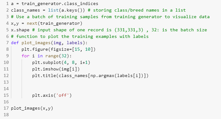
Visualize train image samples with corresponding labels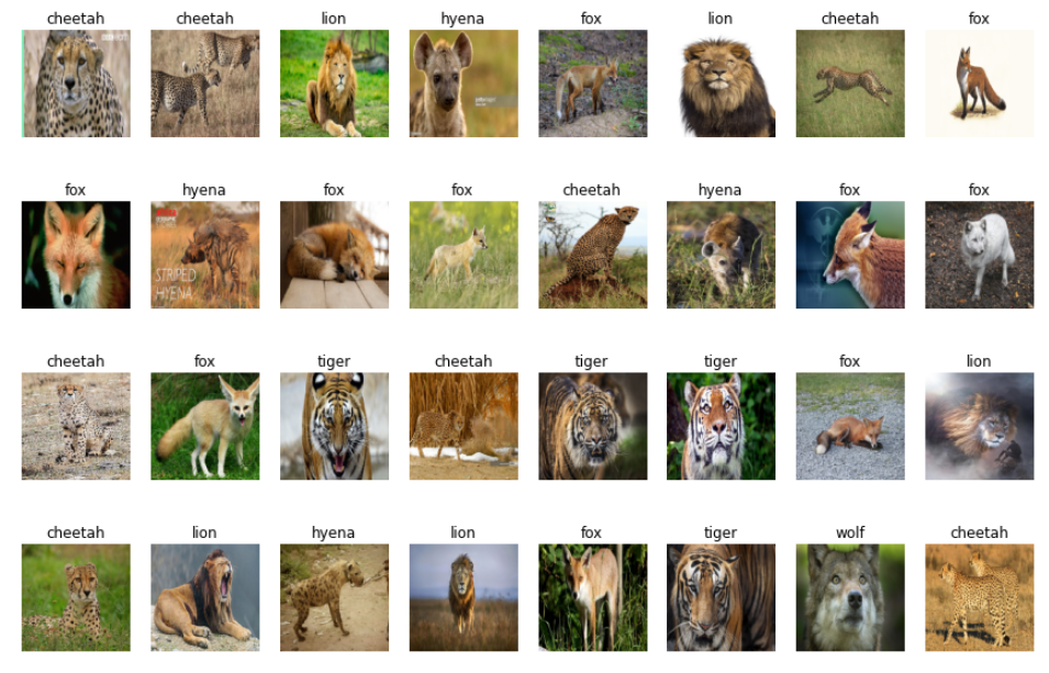
Load the base model(InceptionResNetV2 architecture). Freeze the internal layers of the base model i.e, internal state will not change during training. Due to this, the model's trainable weights will not be updated during training. The pre-trained model weights are used as is for internal layers.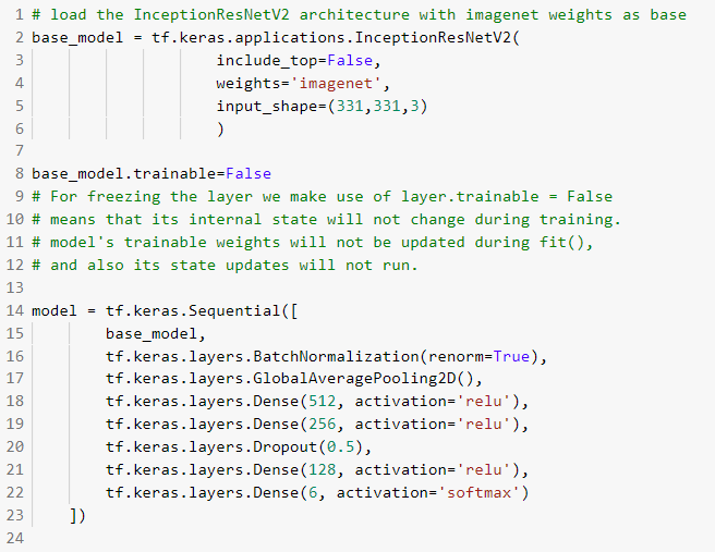
Compile the model by defining optimizer as 'Adam', loss function as 'categorical_crossentropy' and performance metric as 'Accuracy' before training the model. Visualize the model summary.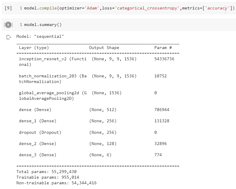
Train the model using early stopping to prevent overfitting.
Early stopping is a method that allows you to specify an arbitrarily large number of training epochs and stop training once the model performance stops improving on the validation dataset. Train the model by passing train data, validation data, number of epochs as 25, callback as early stopping and steps for each epoch.
![]()
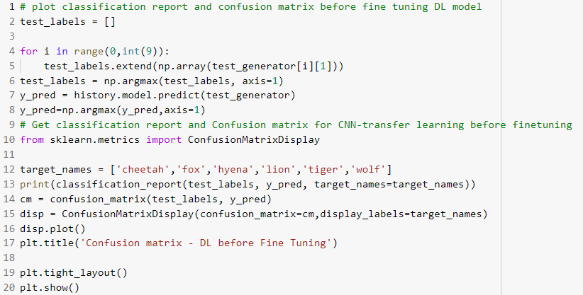
Get test predictions using the trained model.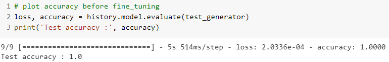 Visualize the performance on test data using classification report and confusion matrix
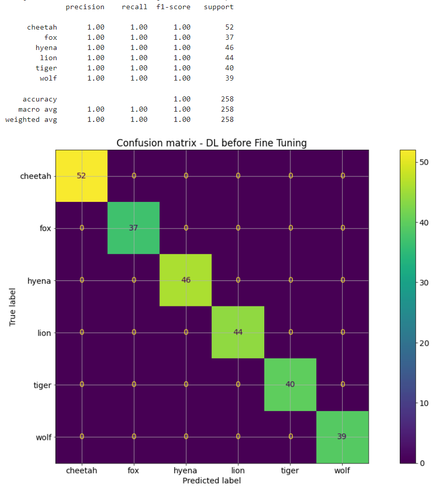
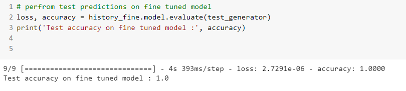
Note that we have achieved 100% accuracy on test data by using very efficient base model along with using early stopping during training to avoid overfitting. Also note that we have stratified our train, validation and test datasets based on class labels. This ensures that each partition as equal distribution of class labels.
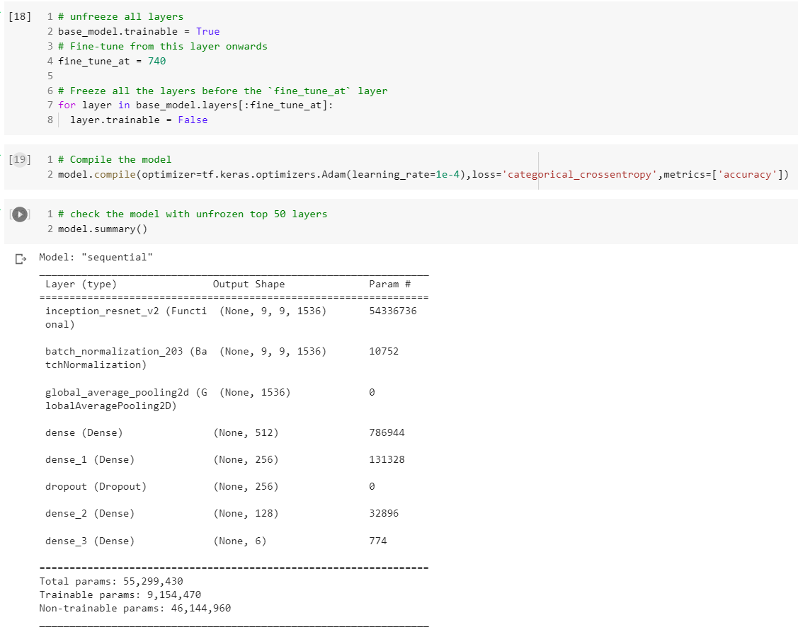
In this part, we are performing fine tuning on InceptionResNetV2 pre-trained model by unfreezing top layers of the base model.
In the previous part, we trained model for image classifier by using Transfer Learning on InceptionResNetV2 pre-trained model without updating the weights of the pre-trained network. In this experiment, we will check the performance by unfreezing the weights of top layers of the pre-trained model alongside the training of the classifier. The first few layers learn very simple and generic features that generalize to almost all types of images. As you go higher up, the features are increasingly more specific to the dataset on which the model was trained. The goal of fine-tuning is to adapt these specialized features to work with the new dataset, rather than overwrite the generic learning.
Here, we are unfreezing top 34 layers of the base model. Recompile the model and visualize the summary report of the model.
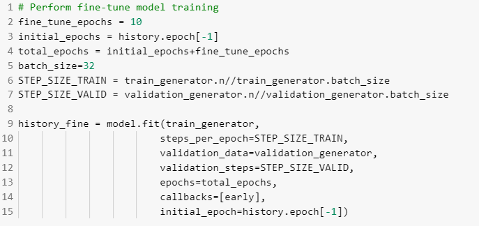
Train the model with fine tuning
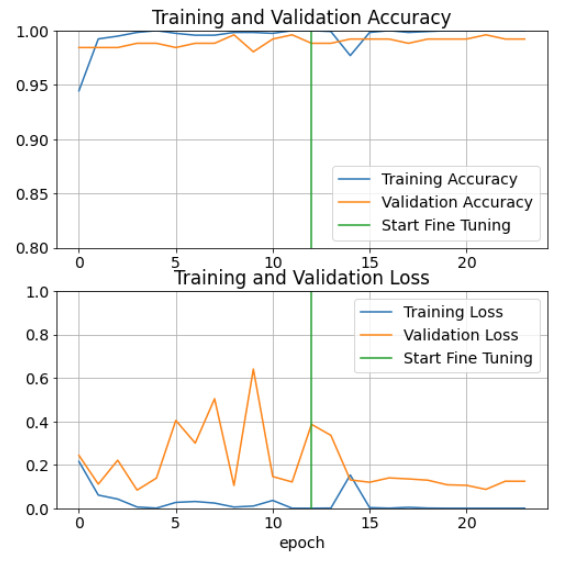
Visualize the performance accuracy curves of train and validation data 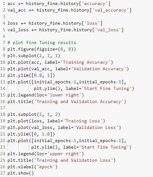
Evaluate the model with fine tuning
 Visualize the performance of fine tuned model on test data using classification report and confusion matrix
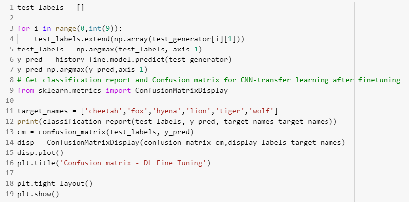
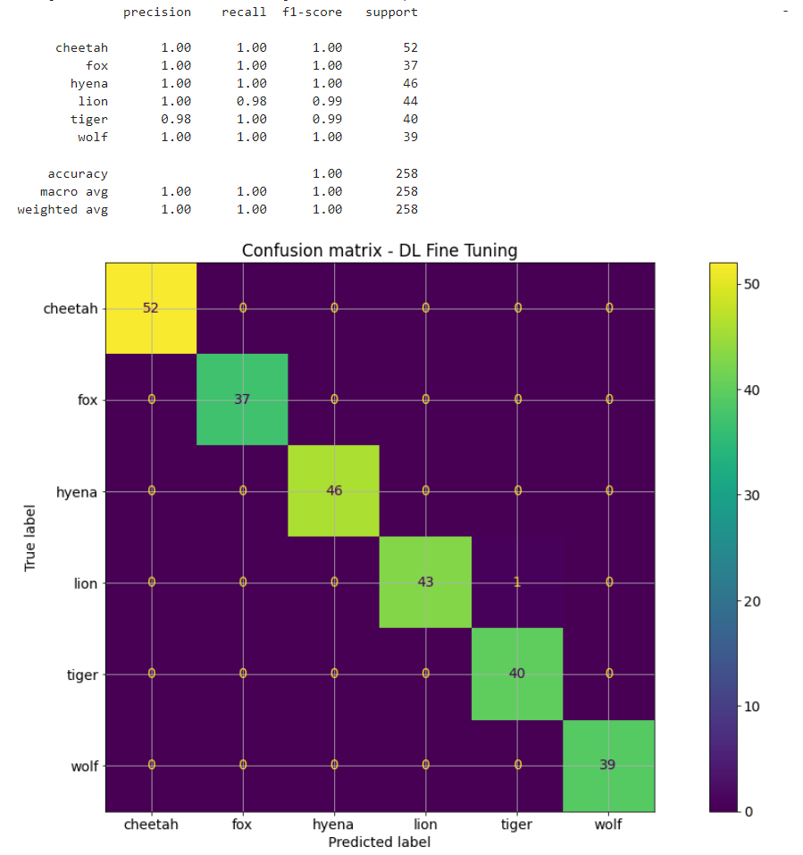
Note that the pre-trained with fine tuning did not help in improving performance accuracy on test data whereas the training curves shows improvement in reduction of training and validation loss.
In this part, we will look at the implementation of multi class image classifier using image features (Bag of Visual Words) with traditional machine learning algorithms like KNN, Naive Bayes, Random Forest and Support Vector Machine classifiers for Wild Animals Images Dataset (Kaggle) [1].
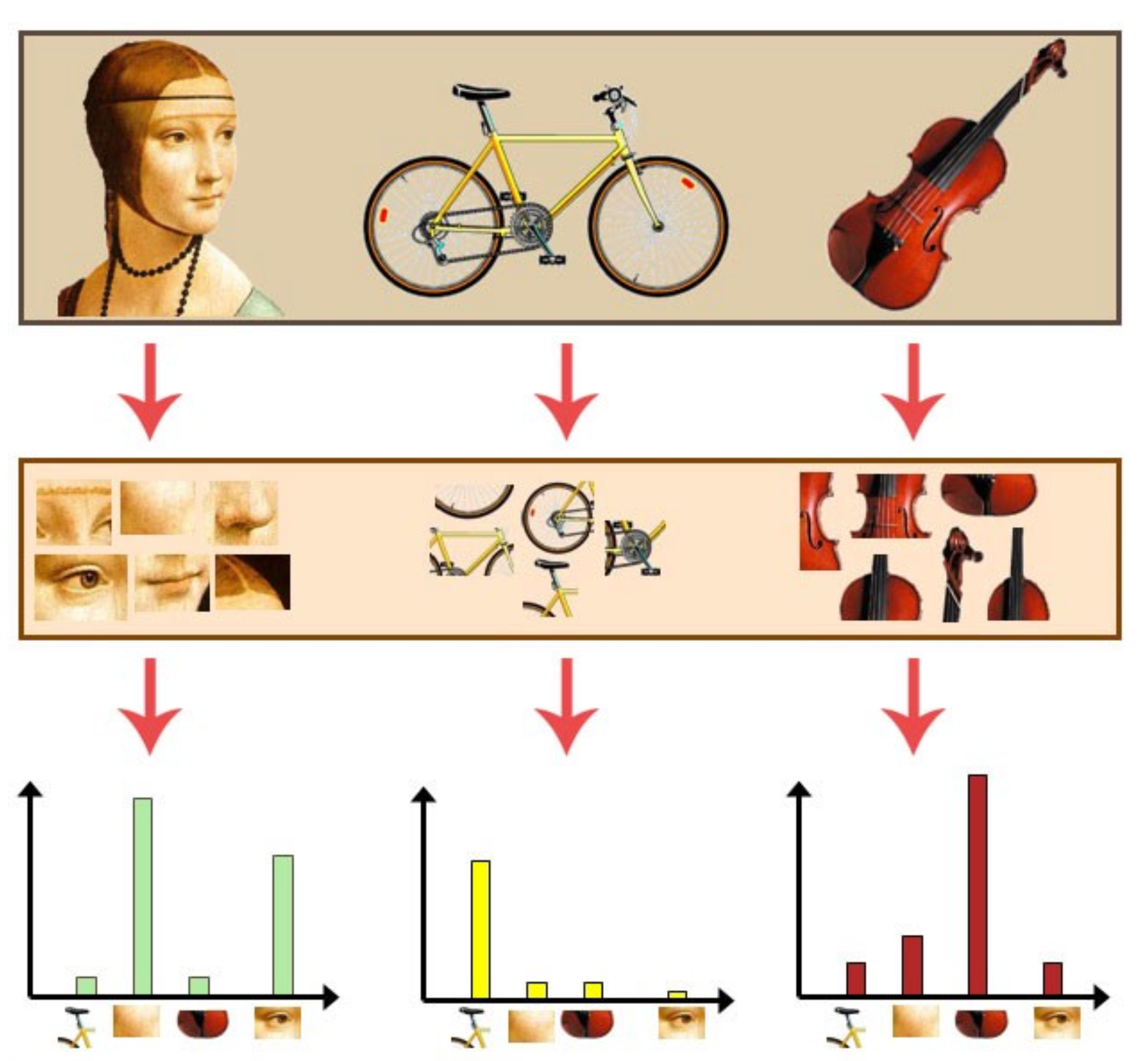
Bag of visual words (BOVW) is commonly used in image classification. Its concept is adapted from information retrieval and NLP’s bag of words (BOW).
The general idea of bag of visual words (BOVW) is to represent an image as a set of features. Features consists of keypoints and descriptors. Keypoints are the “stand out” points in an image, so no matter the image is rotated, shrunk, or expanded, its keypoints will always be the same. And descriptor is the description of the keypoint. We use the keypoints and descriptors to construct vocabularies and represent each image as a frequency histogram of features that are in the image. From the frequency histogram, later, we can find another similar images or predict the category of the image.
1. Extract Bag of Visual Words from images
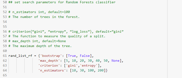
2. Set search parameters for each classifier to identify best hyper parameter values
3. Train the model
4. Evaluate the model
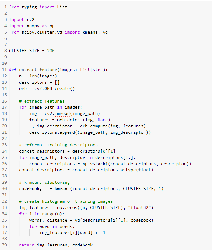
In this step we will extract the image features using Bag of Visual Words. Initially, extract the ORB (Oriented FAST and Rotated BRIEF) descriptors from images. Cluster the extracted descriptors from images using k-means clustering machine learning algorithm. Generate codebook of visual words by extracting the cluster centers. Create the histogram of frequency of occurrence of visual words for training images by assigning the extracted image descriptors from every image in to identified clusters.
Random search parameters for SVM classifier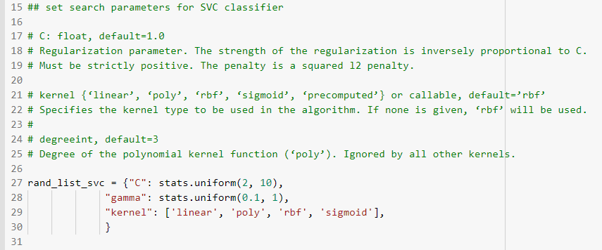 Random search parameters for KNN classifier
 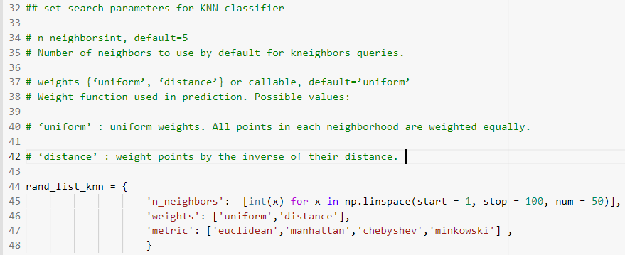 Random search parameters for RF classifier
Define a custom function that performs random search using the provided search space of hyper parameters for every Ml model. The function 'train_models' takes the dictionary of hyper parameter search space, train images, image labels and model_str as parameters.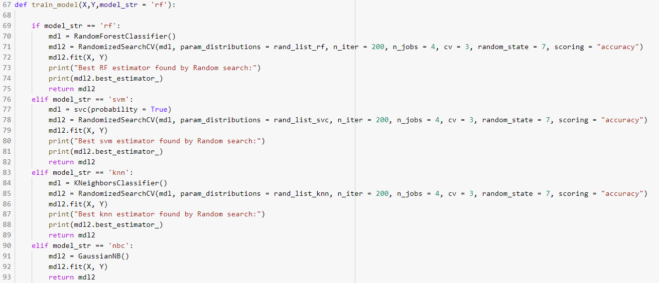
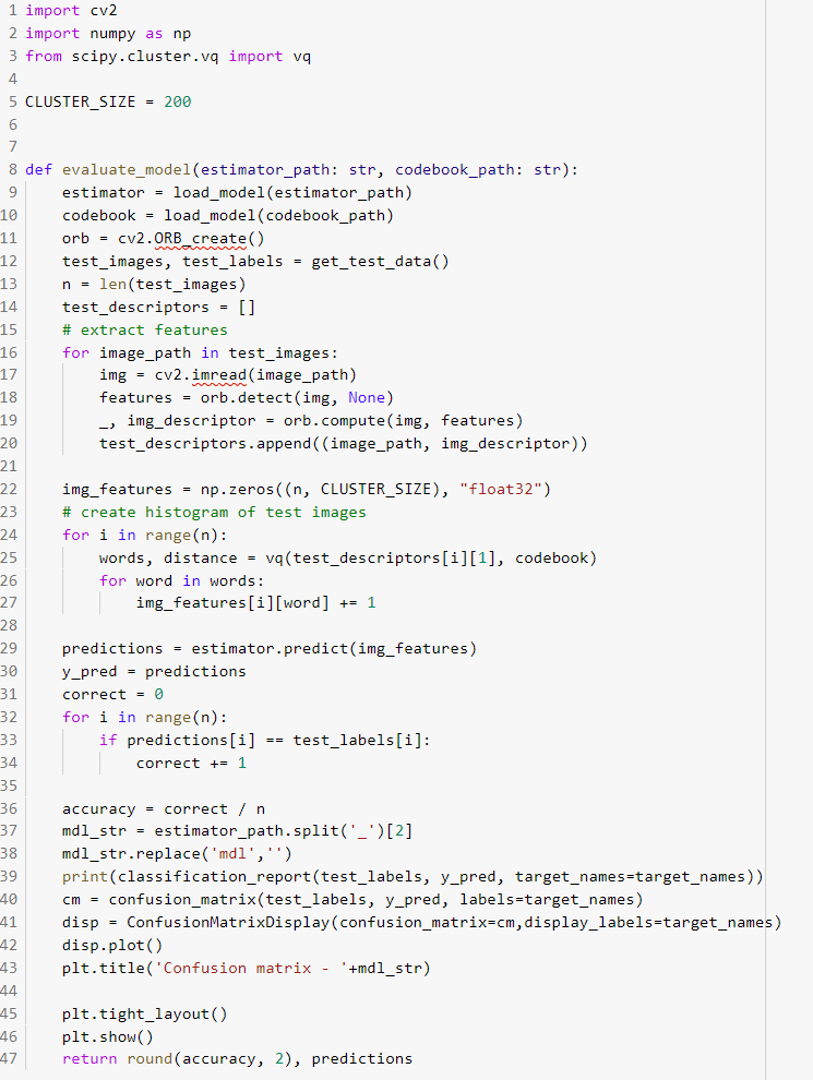
Define an evaluate_model function to perform the following tasks
i. Extract the descriptors for test data
ii. Create test Bag of visual words features from test image descriptors using codebook generated using training data
iii. Generate test predictions using best model and create classification report and confusion matrix to visualize the performance of classifier on test data
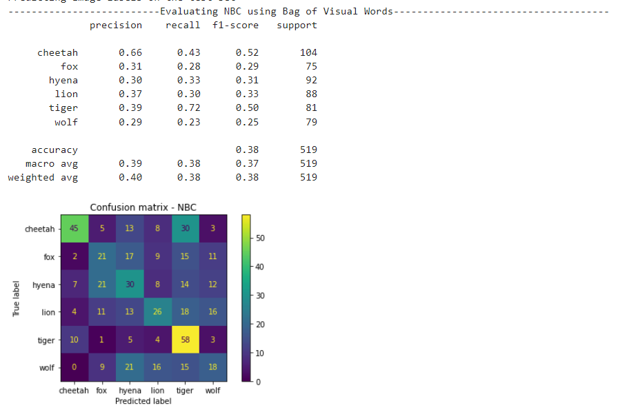
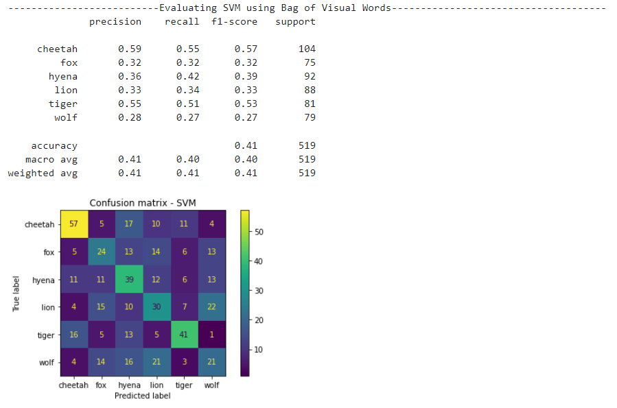
 Visualize the performance on test data by calling 'evaluate_model' for each ML classifier using classification report and confusion matrix.
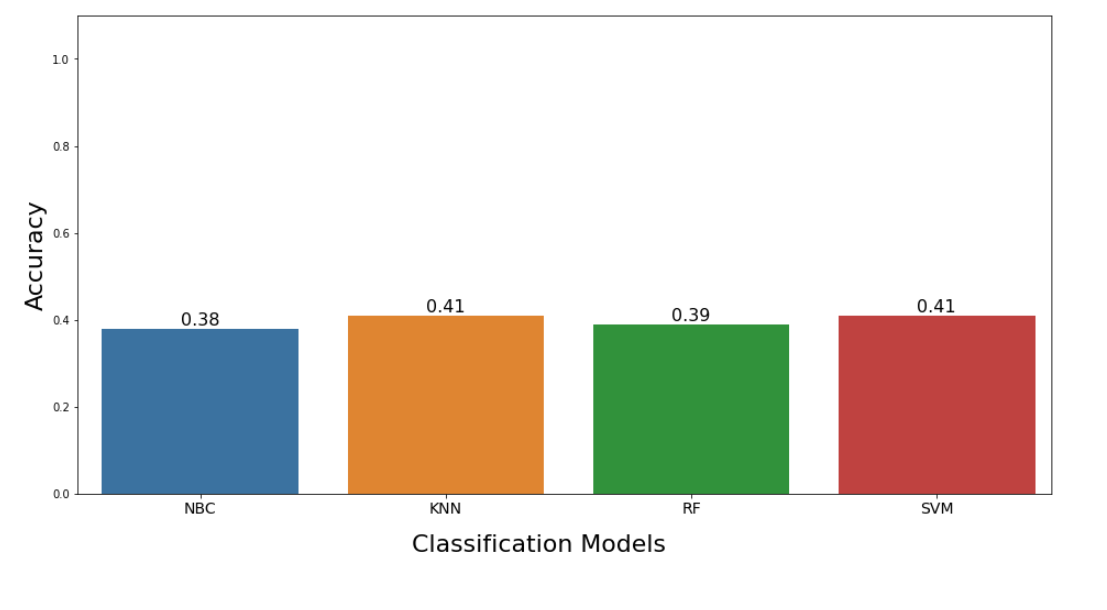 NBC Results
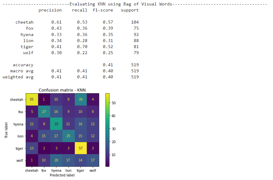
 KNN results
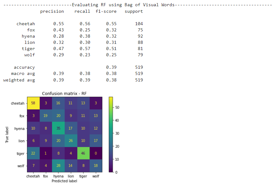
Random Forest results
SVM results
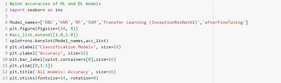
Visualize the comparison of performance between DL and ML methods
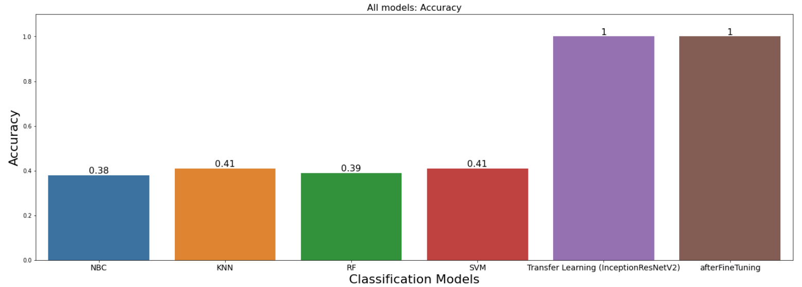
1. The performance improvement is observed when using transfer learning on InceptionResNetV2(pre-trained) model for multi image classification over ML methods using image features (Bag of Visual Words) for Wild Animals Images Dataset (Kaggle) [1].
2. Efficient HPO could help with increasing the performance of certain ML methods. Also, the performance of ML methods depends on the relevance of hand-crafted features extracted to the task at hand.
2. In case of transfer learning, further improvement in reduction of training and validation loss is observed with the use of fine tuning on InceptionResNetV2 pre-trained model by unfreezing top 34 layers of the base model over InceptionResNetV2 pre-trained model without unfreezing top layers .
1.Performed data pre-processing by normalizing the image intensities and performing augmentation using horizontal flip in the case of DL models. Changed the existing folder names and segregated the dataset into separate train and validation/test folders with 70-30 split ratio.
2.Implemented multi-class image classifier using transfer learning on InceptionResNetV2(pre-trained) model and achieved an accuracy score of 100% on test data . (referred tutorial [11])
3. Performed fine tuning on base model by unfreezing top layers (referred tutorial [12]) . Experimented several number of top layers and several learning rate values to achieve best reduction in loss. The achieved accuracy score on test data with fine tuning is 100%.
4. Implemented multi class image classifiers using image features (Bag of Visual Words) with traditional algorithms like KNN, Naive Bayes, Random Forest and Support Vector Machine classifiers (referred tutorial [10,13])
5. Implemented code to identify the best hyper parameter values using random search for SVC classifier, KNN classifier and Random Forest classifier
6. Implemented code to visualize the classification report and confusion matrix for SVC classifier, KNN classifier, NB classifier and Random Forest classifier
7. Compared the performance of ML methods with DL methods using barplot of accuracies.
C hallenge 1: Initially observed high run time for multi class image classifier using transfer learning on InceptionResNetV2 due to the use of CPU
Solution: This problem can be avoided by using the resource of GPU on google colab
Challenge 2: Initially observed difficulty in identifying the best hyper parameter values ML classifier
Solution: This problem can be avoided by using random search parameter values
Challenge 3: Faced challenge in obtaining the image features to use in traditional ML algorithms
Solution: Performed literature review. Understood and implemented Bag Of Visual Words to extract image features
Challenge 4: There are many image classification models use as baseline model in transfer learning
Solution: Performed literature review and chose INceptionResNetV2 as it is the best performing model compared to other networks.
[1] https://www.kaggle.com/datasets/whenamancodes/wild-animals-images
[3] https://medium.com/@anuuz.soni/advantages-and-disadvantages-of-knn-ee06599b9336
[4] https://www.upgrad.com/blog/gaussian-naive-bayes/
[5] https://shubh-tripathi.medium.com/naive-bayes-classifiers-f897eca83e2c
[6] https://www.analyticsvidhya.com/blog/2021/06/understanding-random-forest/
[7] https://www.kdnuggets.com/2022/02/random-forest-decision-tree-key-differences.html
[8] https://www.mygreatlearning.com/blog/random-forest-algorithm/
[10] https://towardsdatascience.com/bag-of-visual-words-in-a-nutshell-9ceea97ce0fb
[11] https://www.geeksforgeeks.org/multiclass-image-classification-using-transfer-learning/
[12] https://www.tensorflow.org/tutorials/images/transfer_learning
created with
Website Builder .